Bloch Sphere: Qubit Visualization

Index

• Quantum States
• Bloch Sphere
• Visualizing a Quantum State
  • 1. Required Dependencies
  • 2. Generating a Random State
  • 3. Displaying the state and Bloch Sphere
• Deriving the Equation
  • Polar Coordinates
  • Simplifying the Vector
• Polar Coordinates on a Sphere
• Half-Angles
• Conclusion

Quantum States

In quantum computing, the possible states of a system can be mathematically represented as a linear combination of the vectors ∣ 0 \ket 0 ∣0 and ∣ 1 \ket 1 ∣1 .

Considering a system with only one quantum bit (qubit), we have:

∣ ψ = α ∣ 0 + β ∣ 1 \ket \psi = \alpha \ket 0 + \beta \ket 1 ∣ψ=α∣0+β∣1

Where α , β ∈ C \alpha, \beta \in \mathbb{C} α,β∈C .

---

Bloch Sphere

Without physical meaning, it is a mathematical model used to geometrically represent the state of a qubit, as shown below for the state ∣ 0 \ket 0 ∣0 :

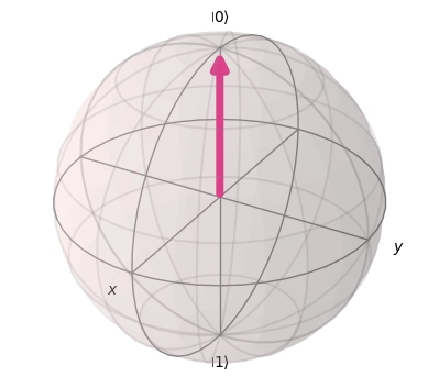
Useful for verifying states in superposition, it can be used to visualize the application of logical operators through the rotation of the state vector.

To be represented on the Sphere, a quantum state can be rewritten in terms of a pair of angles:

∣ ψ = cos ⁡ θ 2 ∣ 0 + e i ϕ sin ⁡ θ 2 ∣ 1 \ket \psi = \cos\frac \theta 2 \ket 0 + e^{i\phi}\sin\frac \theta 2 \ket 1 ∣ψ=cos2θ​∣0+eiϕsin2θ​∣1

---

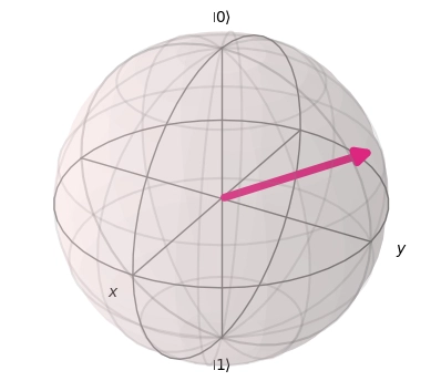
Visualizing a Quantum State

Using Qiskit, a development kit written by IBM to create and manipulate quantum states and circuits in Python, it is possible to generate a random state (using the relation above) and visualize the generated vector on the Bloch Sphere.

1. Required Dependencies

• NumPy: For angle calculations.
• Qiskit: For state generation and Bloch sphere rendering.
• Interactive Environment (e.g., Jupyter Notebook): For image display.
• Matplotlib: Required by Qiskit for plotting.

<span>$ </span>pip <span>install </span>numpy matplotlib qiskit ipykernel
<span>$ </span>pip <span>install </span>numpy matplotlib qiskit ipykernel
$ pip install numpy matplotlib qiskit ipykernel

Enter fullscreen mode Exit fullscreen mode

<span>import</span> <span>numpy</span> <span>as</span> <span>np</span>
<span>from</span> <span>qiskit.quantum_info</span> <span>import</span> <span>Statevector</span>
<span>from</span> <span>qiskit.visualization</span> <span>import</span> <span>plot_bloch_multivector</span>
<span>import</span> <span>numpy</span> <span>as</span> <span>np</span>
<span>from</span> <span>qiskit.quantum_info</span> <span>import</span> <span>Statevector</span>
<span>from</span> <span>qiskit.visualization</span> <span>import</span> <span>plot_bloch_multivector</span>
import numpy as np
from qiskit.quantum_info import Statevector
from qiskit.visualization import plot_bloch_multivector

Enter fullscreen mode Exit fullscreen mode

2. Generating a Random State

First, we can use NumPy methods to create the angles θ \theta θ and ϕ \phi ϕ :

<span>theta</span> <span>=</span> <span>np</span><span>.</span><span>random</span><span>.</span><span>uniform</span><span>(</span><span>0</span><span>,</span> <span>np</span><span>.</span><span>pi</span><span>)</span>
<span>phi</span>   <span>=</span> <span>np</span><span>.</span><span>random</span><span>.</span><span>uniform</span><span>(</span><span>0</span><span>,</span> <span>2</span><span>*</span><span>np</span><span>.</span><span>pi</span><span>)</span>
<span>theta</span> <span>=</span> <span>np</span><span>.</span><span>random</span><span>.</span><span>uniform</span><span>(</span><span>0</span><span>,</span> <span>np</span><span>.</span><span>pi</span><span>)</span>
<span>phi</span>   <span>=</span> <span>np</span><span>.</span><span>random</span><span>.</span><span>uniform</span><span>(</span><span>0</span><span>,</span> <span>2</span><span>*</span><span>np</span><span>.</span><span>pi</span><span>)</span>
theta = np.random.uniform(0, np.pi)
phi   = np.random.uniform(0, 2*np.pi)

Enter fullscreen mode Exit fullscreen mode

The angle limitations will be explained later.

With the angles, we create a Statevector from a list, where the first element represents the ∣ 0 \ket 0 ∣0 portion of the vector, and the second represents the ∣ 1 \ket 1 ∣1 portion:

<span>state</span> <span>=</span> <span>Statevector</span><span>([</span>
    <span>np</span><span>.</span><span>cos</span><span>(</span><span>theta</span><span>/</span><span>2</span><span>),</span>
    <span>np</span><span>.</span><span>exp</span><span>(</span><span>phi</span> <span>*</span> <span>1.j</span><span>)</span> <span>*</span> <span>np</span><span>.</span><span>sin</span><span>(</span><span>theta</span><span>/</span><span>2</span><span>)</span>
<span>])</span>
<span>state</span> <span>=</span> <span>Statevector</span><span>([</span>
    <span>np</span><span>.</span><span>cos</span><span>(</span><span>theta</span><span>/</span><span>2</span><span>),</span>
    <span>np</span><span>.</span><span>exp</span><span>(</span><span>phi</span> <span>*</span> <span>1.j</span><span>)</span> <span>*</span> <span>np</span><span>.</span><span>sin</span><span>(</span><span>theta</span><span>/</span><span>2</span><span>)</span>
<span>])</span>
state = Statevector([
    np.cos(theta/2),
    np.exp(phi * 1.j) * np.sin(theta/2)
])

Enter fullscreen mode Exit fullscreen mode

Note: since in computing i is a commonly used letter, the complex root is represented by j.

3. Displaying the state and Bloch Sphere

By executing this code in Jupyter cells, we can display the results of the operations

• writing the state created by Statevector in text or LaTeX format
• illustrating the Sphere as an image

<span>display</span><span>(</span><span>state</span><span>.</span><span>draw</span><span>(</span><span>'</span><span>LaTeX</span><span>'</span><span>))</span>
<span>plot_bloch_multivector</span><span>(</span><span>state</span><span>)</span>
<span>display</span><span>(</span><span>state</span><span>.</span><span>draw</span><span>(</span><span>'</span><span>LaTeX</span><span>'</span><span>))</span>
<span>plot_bloch_multivector</span><span>(</span><span>state</span><span>)</span>
display(state.draw('LaTeX'))
plot_bloch_multivector(state)

Enter fullscreen mode Exit fullscreen mode

An example output would be:

0.7727507428 ∣ 0 + ( − 0.4500494484 + 0.4475620442 i ) ∣ 1 0.7727507428 \ket 0 + (−0.4500494484 + 0.4475620442 i)\ket 1 0.7727507428∣0+(−0.4500494484+0.4475620442i)∣1

---

Deriving the Equation

Let’s deduce the equation, showing in a simplified manner why it is valid.

Polar Coordinates

Let z z z be a complex number, such that z = x + i y z = x + iy z=x+iy (where i i i is the imaginary unit).

This number can be represented in the Argand-Gauss plane as a vector with modulus ρ \rho ρ :

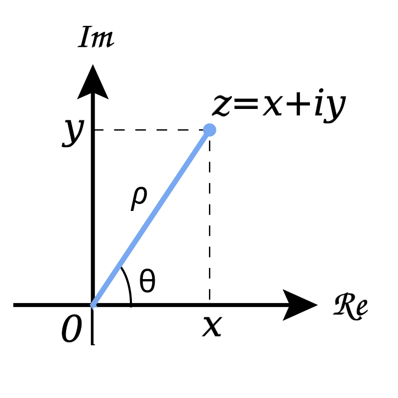
We can represent the vector in its polar form, rewriting its sides in terms of the angle between them:

x = ρ cos ⁡ θ y = ρ sin ⁡ θ ∴ z = ρ cos ⁡ θ + i ρ sin ⁡ θ z = ρ ( cos ⁡ θ + i sin ⁡ θ ) x = \rho\cos\theta \\ y = \rho\sin\theta \\ \therefore z = \rho\cos\theta + i\rho\sin\theta \\ z = \rho(\cos\theta + i\sin\theta) x=ρcosθy=ρsinθ∴z=ρcosθ+iρsinθz=ρ(cosθ+isinθ)

Applying Euler’s Formula, we have:

z = ρ e i θ z = \rho e^{i\theta} z=ρeiθ

Thus, we can rewrite the state vector ψ \psi ψ as:

∣ ψ = ρ 0 e i θ 0 ∣ 0 + ρ 1 e i θ 1 ∣ 1 \ket\psi = \rho_0e^{i\theta_0}\ket 0 + \rho_1e^{i\theta_1}\ket 1 ∣ψ=ρ0​eiθ0​∣0+ρ1​eiθ1​∣1

Simplifying the Vector

In summary, the “global phase” is a mathematical representation of the phase of a quantum system, consisting of a factor that multiplies a state without altering its physical properties.

That is, we can multiply the state vector by its global phase while maintaining the described relations:

∣ ψ ′ = e − i θ 0 ∣ 0 ∣ ψ ′ = ρ 0 ∣ 0 + ρ 1 e i ( θ 1 − θ 0 ) ∣ 1 \ket{\psi’} = e^{-i\theta_0}\ket 0 \\ \ket{\psi’} = \rho_0\ket 0 + \rho_1e^{i(\theta_1-\theta_0)}\ket 1 ∣ψ′=e−iθ0​∣0∣ψ′=ρ0​∣0+ρ1​ei(θ1​−θ0​)∣1

Let θ = θ 1 − θ 0 \theta = \theta_1 – \theta_0 θ=θ1​−θ0​ :

∣ ψ ′ = ρ 0 ∣ 0 + ρ 1 e i θ ∣ 1 \ket{\psi’} = \rho_0\ket 0 + \rho_1e^{i\theta}\ket 1 ∣ψ′=ρ0​∣0+ρ1​eiθ∣1

We can also rewrite one of the coefficients in the form x + i y x + iy x+iy , since the original coefficients ( α \alpha α and β \beta β ) are complex:

β = ρ 1 e i θ = x + i y \beta = \rho_1e^{i\theta} = x + iy β=ρ1​eiθ=x+iy

As this notation is equivalent to the original, the vector remains normalized, that is:

∣ ρ 0 ∣ 2 + ∣ x + i y ∣ 2 = 1 ρ 0 2 + x 2 + y 2 = 1 |\rho_0|^2 + |x + iy|^2 = 1 \\ \rho_0^2 + x^2 + y^2 = 1 ∣ρ0​∣2+∣x+iy∣2=1ρ02​+x2+y2=1

This last equation represents a sphere in a three-dimensional space, meaning that the state vector can be represented on a sphere.

Polar Coordinates on a Sphere

Analogous to a two-dimensional vector, a three-dimensional vector ( x , y , z x, y, z x,y,z ) on a sphere can have its components written in polar form as:

x = ρ sin ⁡ θ cos ⁡ ϕ y = ρ sin ⁡ θ sin ⁡ ϕ z = ρ cos ⁡ θ x = \rho\sin\theta\cos\phi \\ y = \rho\sin\theta\sin\phi \\ z = \rho\cos\theta x=ρsinθcosϕy=ρsinθsinϕz=ρcosθ

Where:

• θ \theta θ is the angle formed between the vector and the z z z axis;
• ϕ \phi ϕ is the angle formed between the vector and the x x x axis;
• ρ 0 = z \rho_0 = z ρ0​=z ;
• Normalization ensures that ρ = 1 \rho = 1 ρ=1 .

Rewriting the vector in polar coordinates, we have:

∣ ψ ′ = z ∣ 0 + ( x + i y ) ∣ 1 ∣ ψ ′ = cos ⁡ θ ∣ 0 + sin ⁡ θ ( cos ⁡ ϕ + i sin ⁡ ϕ ) ∣ 1 ∣ ψ ′ = cos ⁡ θ ∣ 0 + e i ϕ sin ⁡ θ ∣ 1 \ket{\psi’} = z\ket 0 + (x+iy)\ket 1 \\ \ket{\psi’} = \cos\theta\ket 0 + \sin\theta(\cos\phi+i\sin\phi)\ket 1 \\ \ket{\psi’} = \cos\theta\ket 0 + e^{i\phi}\sin\theta\ket 1 ∣ψ′=z∣0+(x+iy)∣1∣ψ′=cosθ∣0+sinθ(cosϕ+isinϕ)∣1∣ψ′=cosθ∣0+eiϕsinθ∣1

Half Angles

However, this is not the complete Sphere. To be able to represent any state vector, we restrict the angles such that:

• 0 ≤ θ ≤ π 0 \leq \theta \leq \pi 0≤θ≤π
• 0 ≤ ϕ ≤ 2 π 0 \leq \phi \leq 2\pi 0≤ϕ≤2π

Thus, we arrive at the general form of a quantum state vector as a function of its angles:

∣ ψ = cos ⁡ θ 2 ∣ 0 + e i ϕ sin ⁡ θ 2 ∣ 1 \ket \psi = \cos\frac \theta 2 \ket 0 + e^{i\phi}\sin\frac \theta 2 \ket 1 ∣ψ=cos2θ​∣0+eiϕsin2θ​∣1

---

Conclusion

Using this relation, we ensure that the generated state can always be visualized on a Bloch Sphere, which implies that it will always be a valid state.

原文链接：Bloch Sphere: Qubit Visualization