Note: This post was originally published on https://bignumworks.com
Introduction
In this article, we will explore how to analyze time series data with Python’s Pandas Data Analysis library.
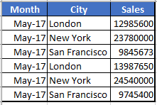
Let’s first understand what we mean by Time Series data. In simple terms, time series represent a set of observations taken over a period of time. It occurs whenever the data is recorded on a regular basis. For example…
Here, we have a Sales data recorded over months for multiple locations.
Time series data analysis is extremely important for making informed business and policy decisions and plans. It is used to
- find out the past trends
- use the past trends to forecast current future trends.
- find out cyclic variations
- discover seasonal variations
For example, a retailer can discover the seasonal and cyclic sales trends of it’s inventory and plan accordingly.
Our Methodology
- We will start with importing the necessary python modules.
- And then we will read in a dataset having time series data.
- We will transform the data to make sure it is indexable on the time series data column.
- We will then demonstrate how to select and filter data based on date and time.
- And finally we will visualize the time series data.
Setting up your machine
For the code demo in this article, we are using Python 3.x and Python modules Pandas and matplotlib. We are using Pandas for reading in the data and data analysis and matplotlib for data visualization. The best way to get all the required is by installing Anaconda Data Science Python Districtuion.
Importing Python Modules
We start with importing Pandas, matplotlib and datetime modules. We are importing datetime module for as we would need to use some of it’s methods. We are also setting matplotlib inline to make sure the plots are shown right in the Jupyter Notebook
from datetime import datetime
import pandas as pd
%matplotlib inline
import matplotlib.pyplot as pyplot
Introducing our dataset
For this code demo, we are creating a sample employees dataset with two columns
- Date field
- No of Employees
This data is a quarterly count of employees from last 8 quarters.
We create a data dictionary with columns names a keys and records as the values. We then pass this dict object to Pandas DataFrame method and create a DataFrame where this data will be stored in tabular format.
employees = {'Date': ['2015-09-30', '2015-12-31', '2016-03-31', '2016-06-30',
                 '2016-09-30', '2016-12-31', '2017-03-31', '2017-06-30'],
        'Employees': [9, 15, 26, 15, 15, 14, 26, 25]}
df = pd.DataFrame(employees, columns = ['Date', 'Employees'])
Now, we have our data in a Pandas DataFrame, let’s print it out to see how it looks.
print(df)
         Date  Employees
0  2015-09-30          9
1  2015-12-31         15
2  2016-03-31         26
3  2016-06-30         15
4  2016-09-30         15
5  2016-12-31         14
6  2017-03-31         26
7  2017-06-30         25
As we can see, we have the data with two columns Date and Employees. Also, notice that there is a numeric row index which has been set automatically while importing data into a DataFrame. We would have to change this later.
Pandas Time and Date methods
let’s get some information about the dataset, like datatypes of the column
df.info()
<class 'pandas.core.frame.DataFrame'>
RangeIndex: 8 entries, 0 to 7
Data columns (total 2 columns):
Date         8 non-null object
Employees    8 non-null int64
dtypes: int64(1), object(1)
memory usage: 136.0+ bytes
We see that the date column is object, which means it’s stored as text. Date time data in text format in not very useful for running time series analysis. We need to first convert this to a datetime datatype
We do this conversion by calling Pandas to_datetime method on the date column. We assign the converted date column back to the original Pandas DataFrame, thereby replacing the old text date column with the new datetime type column.
df['Date'] = pd.to_datetime(df['Date'])
We check the conversion to a datetime datatype by calling the info method again on our DataFrame
df.info()
<class 'pandas.core.frame.DataFrame'>
RangeIndex: 8 entries, 0 to 7
Data columns (total 2 columns):
Date         8 non-null datetime64[ns]
Employees    8 non-null int64
dtypes: datetime64[ns](1), int64(1)
memory usage: 168.0 bytes
And we see that the date column now shows up as datetime datatype.
There is one more thing we need to do before we can start exploring the time series properties. We need to setup the index of our DataFrame to the date column. We do this by calling index on the Pandas DataFrame and assigning it the date series. We also delete the date column as we don’t need it separately from the index.
df.index = df['Date']
del df['Date']
Let’s print out the DataFrame to see how it looks after setting index to date column
print(df)
            Employees
Date
2015-09-30          9
2015-12-31         15
2016-03-31         26
2016-06-30         15
2016-09-30         15
2016-12-31         14
2017-03-31         26
2017-06-30         25
Querying time series data
Now we are set to start exploring our time series data. We will start with showing some data querying techniques.
Here we are querying and filtering the data and selecting only those records that are from year 2016
df['2016']
| Employees | |
|---|---|
| Date | |
| 2016-03-31 | 26 |
| 2016-06-30 | 15 |
| 2016-09-30 | 15 |
| 2016-12-31 | 14 |
Notice that due to our converting the Date column to datetime and setting it as index, we can run all kinds of queries. Above we just passed 2016 and Pandas understood that we are looking for records from year 2016.
Next we are selecting all records from June 2016 onwards.
df[datetime(2016, 6, 30):]
| Employees | |
|---|---|
| Date | |
| 2016-06-30 | 15 |
| 2016-09-30 | 15 |
| 2016-12-31 | 14 |
| 2017-03-31 | 26 |
| 2017-06-30 | 25 |
Time Series data visualized
Here we are using time series to visualize our data by calling the plot method on the DataFrame. Since, we have time series already set as index, we had to simply call the plot method in it’s simplest form to get this plot.
df.plot();
Conclusion
We touch on some of the Pandas time series data analysis capabilities. We transformed and manipulated a dataset containing time series data. We converted it to proper times series format using Pandas in-built methods. We then learned how to explore and filter the data using Pandas date time data methods and functionality. Finally, we saw an easy way to visualize time series data














暂无评论内容